mdC
memoria digital de Canarias
2
o
ANIVERSARIO
2003 2023
2003 2023
mdC

Descargar y escuchar, mientras hacemos otras cosas.
En cualquier parte y sin conexión.
Publicaciones seriadas de Canarias de estimable valor y significativo contenido en el ámbito de la investigación y los estudios locales.
Ver colección
Los textos de ayer y hoy adaptados
para descargar y leer cómodamente.
Memoria digital de Canarias (mdC) ofrece acceso a todo tipo de documentación impresa o manuscrita, gráfica y multimedia.
Textos Imágenes Multimedia
Archivo histórico de la Real Sociedad Económica de Amigos del País de Gran Canaria.
Ver colección
En el año 2004, don Jaime O'Shanahan Bravo de Laguna donó su archivo fotográfico a la Universidad de Las Palmas de Gran Canaria.
Ver colección
Presenta los materiales recolectados por Maximiano Trapero en las Islas Canarias referidos a la literatura oral.
Ver colección
Recuperando el patrimonio intangible tradicional de la capital grancanaria, caracterizado por su pasado cosmopolita y aportación de culturas diversas.
Ver colección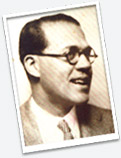
El archivo de este prestigioso arquitecto, está compuesto por más de mil proyectos que reflejan su actividad profesional a lo largo de su vida.
Ver colección
Vida y obra de este singular poeta teldense, una de las más detacadas figuras del modernismo poético canario.
Ver colección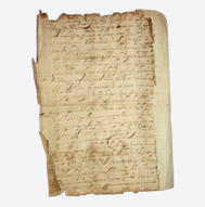
Digitalización y descripción de las 1176 actas, en 5701 imágenes, de las Juntas Generales (1694-1950) y las Juntas de Gobierno internas (1868-1947)
Ver colecciónmanuscritos
libros
artículos de revista
imágenes
audios
vídeos
Las celebraciones forman parte de la etnografía de cada pueblo, como el caso de Canarias. En el Archivo Voces y Ecos encontramos fotografías en blanco y negro sobre celebraciones familiares de las décadas de los años cincuenta y sesenta. Plasman las formas de celebrar diversos eventos familiares como, por ejemplo, Bautismo de la familia García Morera en Guanarteme, Cumpleaños de María Rosa García López o Lola García Morera, Ada García Morera, Felo y Loli López en las Fiestas del Carmen. Relacionado con ello también disponemos en la misma colección de imágenes de los años cincuenta y sesenta, sobre Festivales y salidas donde encontramos fotografías como Inés García con grupo de amigos en Teror, Semana Santa o Fiesta en calle Mayor de Triana. Gracias a estos documentos podemos ver cómo ha variado la forma de divertirnos. De tener que llevar carabina cuando los novios salían o el horario de regreso a casa, hasta la actualidad que ya estas cuestiones han avanzado.
La Biblioteca Insular de Gran Canaria conserva el Fondo de música Orleans, una colección de casi cuatro mil partituras manuscritas e impresas del siglo XIX, pertenecientes a la Casa de Orleans en España y regentada por los Duques de Montpensier. Lothar Siemens Hernández fue el artífice necesario para que el Cabildo Insular de Gran Canaria adquiriese el fondo, señalando su importancia capital por la cantidad de manuscritos, los muchos impresos raros, las ediciones príncipe y encuadernaciones de lujo que contiene, incluyendo la obra de algunos de los mejores compositores de aquel tiempo como Pedro Albéniz, Antonio Luján, Ramón Carnicer, Barbieri, Iradier, Mariano Soriano, Guiseppe Verdi o Donizetti. Entre los documentos de nuestra biblioteca sobre este fondo musicológico está el vídeo documental Sonidos de Orleans realizado por la productora Muak Canarias y producido por CCA Gran Canaria-Centro de Cultura Audiovisual. Cuenta con audios en español, francés e inglés, además de entrevistas a reputadas personalidades expertas en la música, que nos explican la gran valía e importancia de estos documentos.
El paisaje de las Islas Canarias se caracteriza por tener volcanes milenarios, playas desiertas, vertiginosas cascadas, árboles centenarios, campos de lava, piscinas naturales, impresionantes acantilados, profundos barrancos, dunas de arena o frondosos bosques. El archipiélago canario, por razones orográficas, geológicas y climáticas, presenta ecosistemas únicos en el continente europeo, enmarcados dentro de la Región Macaronesia. Se ha de tener en cuenta que es la región española con más parques nacionales. De esta forma cada isla posee sus rincones emblemáticos, muchos de ellos patrimonio de la humanidad, entre ellos: en Tenerife el Parque Nacional del Teide, en Gran Canaria la Reserva Natural de las Dunas de Maspalomas, en El Hierro el Sabinar, en La Palma el Parque Nacional de la Caldera de Taburiente, en La Gomera el Parque Nacional del Garajonay, en Fuerteventura Betancuria, en Lanzarote el Parque Nacional de Timanfaya y en La Graciosa la reserva natural de la Playa de la Cocina.
El archipiélago canario presenta una gran biodiversidad de seres vivos contabilizándose cerca de 15.000 especies. En cuanto a la fauna, los invertebrados son el grupo de seres vivos más diversificado que vive en las islas. Destacan los insectos, que están presentes en todos los medios del archipiélago: el suelo, las rocas, las hojas, las flores, los árboles, los restos de materia orgánica, etc. Respecto a la flora, las plantas constituyen el grupo más numeroso, integrado por musgos, helechos, gimnospermas y angiospermas. Nuestra diversidad biológica aumenta en importancia teniendo en cuenta que muchos de estos seres vivos son autóctonos de Canarias, especies que solo viven en esta región del planeta. De hecho es la región de España que cuenta con mayor número de endemismos. En cuanto al material bibliográfico albergado por este repositorio documental, contamos con múltiples formatos como el multimedia, que ofrece audiovisuales y documentos sonoros sobre esta materia, concretamente de botánica y también para el estudio de la fauna.